Erdős 1016 · jehlp.net

1 Pancyclic graphs

A graph is a set of vertices (dots) joined by edges (lines). Here graphs are simple: no edge joins a vertex to itself, and no pair of vertices has two edges between them. The geometry of the drawing does not matter. Lines that cross do not create new vertices.

A path follows edges without repeating vertices. A graph is connected if a path joins every pair of vertices. Its connected components are the separate maximal connected pieces.

A cycle follows edges back to its starting vertex without visiting any other vertex twice. Its length is its number of edges, also its number of vertices. A graph on $n$ vertices is pancyclic if it contains a cycle of each length $3, 4, \dots, n$ .

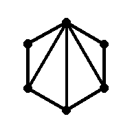
Start with one cycle through all the vertices. Such a cycle is called Hamiltonian; it ensures the graph is connected. Extra edges between its vertices are called chords. Which chords produce cycles of every shorter length?

Six-vertex graph

Select the chords. Then select a cycle length to show an example. The display identifies each missing length.

Write the smallest possible edge count as $n + h (n)$ . The function $h$ measures the excess over the $n$ edges of a Hamiltonian cycle. The theorem states:

h (n) = \log_{2} n + \log^{*} n + O (1)

The notation $O (1)$ means an error bounded by a fixed constant, independent of $n$ . It does not mean approximately one. It does not describe a relative error. More generally, $O (f (r))$ means a quantity whose absolute size is at most a fixed constant times $f (r)$ , for all sufficiently large $r$ . All logarithms below are base two unless written $\ln$ , which means the natural logarithm.

A logarithm reverses exponentiation: $\log_{2} 8 = 3$ because $2^{3} = 8$ . The iterated logarithm $\log^{*} n$ counts how many repeated logarithms take $n$ down to at most 1. Equivalently, define the towers $T_{0} = 1$ and $T_{j + 1} = 2^{T_{j}}$ ; $\log^{*} n$ is the least $j$ with $n \leq T_{j}$ .

Iterated logarithms

Although $\log^{*}$ grows slowly, it is unbounded. A cycle count alone cannot prove that the formula requires this term.

2 Binary shortcuts

First, show that the stated number of edges is sufficient. An upper bound comes from constructing one successful graph. A lower bound, the harder direction here, must constrain every successful graph.

On a large cycle, select consecutive arc segments of lengths $2, 3, 5, 9, \dots, 2^{k - 1} + 1$ . Add a one-edge shortcut across each segment. Each shortcut reduces the length by $1, 2, 4, 8, \dots$ edges, respectively. Every integer from 0 through $2^{k} - 1$ is a sum of a subset of these powers of two. Thus the graph represents binary notation.

Binary shortcut choices

A closing edge joins the two ends of the arc. Select the long segments that the shortcuts replace. The same graph contains every displayed choice.

The complete construction for all lengths

For $n \geq 7$ , select the largest $k$ with $2^{k} + k + 1 \leq n$ . Name the segment endpoints $v_{0}, \dots, v_{k}$ . The original arc has length $2^{k} + k - 1$ . Add the $k$ segment shortcuts. Add the closing edge $v_{0} v_{k}$ .

The arc and its closing edge give all lengths $[k + 1, 2^{k} + k]$ . The arc and the other side of the original $n$ -cycle give $[n - 2^{k} + 1, n]$ . The maximal choice of $k$ implies $n \leq 2^{k + 1} + k + 1$ . Thus at most one length lies between these intervals. If that length is missing, one chord of the original cycle supplies it.

For example, $n = 11$ gives $k = 2$ and intervals $[3, 6]$ and $[8, 11]$ . Only length 7 is missing. To supply it, connect vertices at distance 6 around the original cycle. For $n = 16$ , $k = 3$ gives $[4, 11]$ and $[9, 16]$ . Only length 3 lies below these intervals.

To supply the shorter lengths, start at $t = k$ . While $t > 2$ , set $j = ⌈ \log_{2} t ⌉$ . Add $v_{0} v_{j}$ .

The first $j$ segments give $[j + 1, 2^{j} + j]$ . Because $2^{j} \geq t$ , this interval overlaps the lengths already supplied. Replace $t$ by $j$ . Repeat the procedure until it supplies triangles. The procedure uses at most $\log^{*} k - 1$ further chords.

The ceiling $⌈ x ⌉$ rounds up; the floor $⌊ x ⌋$ rounds down. For $3 \leq n \leq 6$ , use the original cycle. When $n \geq 4$ , add the chord between vertices 0 and 2. When $n = 6$ , also add chord 0–3.

The large case uses at most $k$ segment shortcuts and one closing edge. It also uses at most one gap chord and $(\log^{*} k - 1)$ recursive chords. The total is at most $k + \log^{*} k + 1$ . Since $k \leq ⌊ \log_{2} n ⌋$ and $\log^{*} k \leq \log^{*} n$ , these constructions give the explicit bound

h (n) \leq ⌊ \log_{2} n ⌋ + \log^{*} n + 1

The recursive procedure for shorter lengths suggests why the log-star term occurs. It does not prove that every construction requires this many edges.

3 Cycle space

The degree of a vertex is the number of incident edges. In a cycle, each used vertex has degree two. More generally, an even edge set selects edges so every vertex has even degree. It can be empty, contain several cycles, or have vertices of degree four. It need not be a single cycle.

Add two edge sets by symmetric difference, or XOR: an edge survives exactly when it occurs in one set but not both. At each vertex, even plus even remains even. Thus all even sets form a binary vector space, called the graph’s cycle space. Its scalars are 0 and 1 with $1 + 1 = 0$ .

Combine cycle-space vectors

Two triangles that share one vertex form a basis. Independent on/off choices generate every even set. The two triangles together form an even set, but not one simple cycle.

A cycle-space word is a binary codeword with one parity check at each vertex. XOR adds valid codewords and preserves every parity check. A basis is a list of independent vectors that generates the space uniquely. A space with $r$ binary basis vectors has exactly $2^{r}$ elements. Here $r$ is the cycle rank:

r = edges - vertices + components

Proof of the dimension formula

A tree is a connected graph without any cycle; a forest is a graph without cycles, possibly disconnected. Choose a spanning forest: within each connected component, keep a tree reaching every vertex. If there are $v$ vertices and $c$ components, it has $v - c$ edges.

Each remaining edge forms a unique cycle through the forest. These fundamental cycles are independent because each has its own non-forest edge. They generate every even set: XOR removes its non-forest edges and leaves an even set inside a forest. A forest with an edge has a leaf, a vertex of degree one, so the remaining even set must be empty. There are $e - (v - c)$ fundamental cycles. This proves the formula.

A pancyclic graph is connected. With $n + h$ edges, its rank is $h + 1$ . It requires at least $n - 2$ distinct simple cycles, one for each required length. Each cycle is a nonzero cycle-space word. Thus

\begin{matrix} n - 2 & \leq 2^{h + 1} - 1 \\ h & \geq \log_{2} (n - 1) - 1 \end{matrix}

This is the classical counting lower bound. It gives the term $\log_{2} n$ , but not the additional term $\log^{*} n$ .

4 Normalized length capacity

Simple cycles use only some available words. Different cycles can have the same length. The proof measures how efficiently cycles supply a consecutive interval of lengths. The number of cycles alone does not measure this efficiency.

Suppose a graph of actual rank $r$ contains lengths 3 through $q$ . Its normalized length capacity is $(q - 2) / 2^{r}$ . Define $Φ (R)$ as the supremum (least upper bound) of this quantity over graphs whose actual rank is at least $R$ .

Φ (R) = \sup_{r \geq R} \frac{q - 2}{2^{r}} \leq 1

The denominator always uses the graph’s actual rank, not the cutoff $R$ . A higher cutoff excludes candidates, so $Φ$ cannot increase. Disconnected realizers can be connected by bridges: a bridge joins components and creates no cycle, preserving both rank and the existing lengths.

The goal is $Φ (r) \leq C \cdot 2^{- \log^{*} r}$ for one fixed constant $C$ . Only a slowly decreasing fraction of binary capacity can supply a complete interval of lengths.

Extract a small witness

W

↓Many outside words must be forests↓A random outside word is a forest with probability at most about one half↓Capacity nearly halves at every exponential scale

5 Witness extraction

Inside a graph that already contains a long consecutive interval, build a witness $W$ : a union of selected cycles. Start with the empty set. Find the least length $\geq 3$ that $W$ does not represent. Select a cycle of that length from the host graph. Add its edges. At the first rank $t \geq 2 R$ , stop.

If the old union contained the new cycle, it would already contain that length. Thus the new cycle is not contained in the old union. Because every old edge lies on a cycle, the added cycle increases the rank by at least one. The increase can exceed one. The proof does not assume equality.

Assign each step to the preceding rank. Assign no step to a skipped rank.

At preceding rank $s$ , fewer than $2^{s}$ lengths are present. Thus the least missing length is at most $2^{s} + 2$ . Once $s \geq R$ , the definition of $Φ$ improves this bound to $Φ (R) 2^{s} + 3$ . The sums of these geometric bounds for the same witness give:

\begin{matrix} m \leq 2^{3 R}, c \leq 2 R \\ (m + 1) 2^{- t} \leq Φ (R) + 2^{1 - R} \end{matrix}

Here $m$ is the number of witness edges, $t$ its rank, and $c$ its number of components. Count components only on vertices that the witness uses. Exclude isolated vertices elsewhere in the host.

Check both witness bounds

There are at most $2 R$ selected cycles because every preceding rank is a different integer below $2 R$ . Their union has at most that many components. For sufficiently large $R$ , the sum of coarse length bounds over all possible preceding ranks gives:

\begin{matrix} m & \leq \sum_{s = 0}^{2 R - 1} (2^{s} + 2) \\ = 2^{2 R} + 4 R - 1 \leq 2^{3 R} \end{matrix}

For $s < R$ , use the coarse bound. For subsequent ranks, use the $Φ$ -bound. With $φ = Φ (R)$ , this gives $m + 1 \leq φ 2^{2 R} + 2^{R} + 5 R$ . Because the stopping rank $t$ is at least $2 R$ , division by $2^{t}$ gives $(m + 1) 2^{- t} \leq φ + 2^{1 - R}$ . This bound also requires sufficiently large $R$ . A rank increase can skip terms in these sums, which can only improve the bounds.

The restriction map gives a length bound

Let $M$ be the edges outside $W$ . Restrict each cycle-space word to $M$ . This is a linear map. Its kernel, the words that restrict to the empty set, is exactly the cycle space supported inside $W$ , of dimension $t$ . Thus there are $2^{r - t}$ possible outside words, each with exactly $2^{t}$ preimages. Therefore a uniform ambient word gives a uniform distribution on the image.

A simple cycle that meets both $W$ and $M$ leaves a forest outside. Removal of at least one edge breaks the simple cycle. For a fixed outside word, the number of inside edges ranges from 0 through $m$ . Thus at most $m + 1$ total lengths can occur. A cycle entirely outside contributes at most one length per outside word. Cycles entirely inside contribute at most $m$ possible lengths.

Let $P$ be the probability that a uniform ambient even set restricts to a forest outside. Count these three categories. Divide the count by $2^{r}$ to obtain

\begin{matrix} (q - 2) 2^{- r} & \leq (m + 1) 2^{- t} P \\ + 2^{- t} + m 2^{- r} \end{matrix}

These categories can count some lengths more than once, which preserves an upper bound. The two final terms are small at the scales below. If the host interval is too short to complete the extraction, its normalized capacity is already below the recurrence’s error term.

Removal of some edges from a simple cycle leaves no cycle. Such an edge set is a forest; the empty set counts, but a nonempty path counts too. A fixed outside edge set has a fixed length contribution. The witness can add only 0 through $m$ edges. Thus the same outside word gives at most $m + 1$ total lengths.

XOR and restriction

These two triangles share a diagonal. XOR removes that shared edge. Mark one triangle as $W$ . Examine the edges that remain outside $W$ . With both basis cycles selected, the ambient word is a square, but the outside restriction is a nonempty path.

Triangle 0–1–2 XOR triangle 0–2–3 equals square 0–1–2–3. Removal of witness edges 0–1, 1–2, 0–2 leaves path 2–3–0. Its endpoints have odd degree. It is a forest, although the original word contained a cycle.

The remaining question is: how large can $P$ be?

6 The forest estimate

A forest is any edge set with no cycle, including the empty set. To select a cycle-space word uniformly, generate an independent fair bit for each basis vector. Take the XOR of the basis vectors whose bits are 1. Do not select each edge independently. That usually produces odd degrees.

Do not select a simple cycle uniformly. This probability space includes empty even sets and even sets with multiple cycles.

Random even sets

A bridge joins two triangles. Mark the left triangle as $W$ . The bridge is absent from every even word. Exactly two of the four words leave a forest outside $W$ .

A restriction need not have even degrees. For a square with diagonal 0–2, let $W$ be triangle 0–1–2. The restriction of the square word to the complement is path 2–3–0, a nonempty forest. Thus the event “forest outside” includes more words than the event “empty outside.”

Large-rank bound

For all sufficiently large ranks $r$ , let $G$ be connected and simple, and $W$ a nonempty union of cycles with at most $\sqrt{r}$ edges and at most $(\log_{2} r) / 100$ components. Then

P (forest outside W) \leq \frac{1}{2} + \frac{20}{\log_{2} \log_{2} \log_{2} r}

The hypotheses are essential. The small example explains the definitions and the one-half threshold. It does not test this large-rank theorem. For moderate ranks, the right side can exceed 1, so the estimate gives no useful bound. The proof is asymptotic and requires a uniform sufficiently-large threshold.

Why does the bound approach one half? Parity can connect many distant regions through one shared binary choice. A proof that assumes independent cycle events would omit this dependence. The next four chapters bound the actual dependence.

7 Cut correlations

A region here is the induced graph on a vertex set: retain all edges whose two endpoints lie inside. Its cut $δ A$ consists of edges with just one endpoint inside. A zero-cut event means the random even set selects none of those boundary edges.

For disjoint connected regions $A$ and $B$ , contract each region to one vertex. Contraction preserves the relevant projected cycle-space law. Define their links to be the direct edges between them plus the components left after deleting them that touch both. If there are $ℓ$ links, rank subtraction gives this exact identity:

\frac{P (δ A = δ B = 0)}{P (δ A = 0) P (δ B = 0)} = 2^{ℓ - 1}

The notation $δ A = 0$ describes the selected boundary edges. The original graph can still have a nonempty cut. The ratio measures correlation: 1 is independence, above 1 means simultaneous occurrence is more likely than the product predicts. With one link, the ratio is 1; with two links, it is 2; with three links, it is 4. Pairs with at least three links are called exceptional.

Three links have one shared constraint. The four even words are the empty set and the three pairs of paths. Either zero-cut event occurs only in the empty word. Each probability is

1 / 4

, and the joint probability is also

1 / 4

. The correlation ratio is

(1 / 4) \div (1 / 4 \times 1 / 4) = 4

, exactly

2^{3 - 1}

Parallel links

Each route has its own middle vertex. Examine every even word. As the number of links increases, observe the dependence between the two boundary events.

A bound on disjoint exceptional partners

Fix a region with cut size $d$ . After contraction, append its $d$ incident edges as terminal leaves to a spanning forest of the rest. Remove branches that contain no terminal. Three or more links to another contracted region require a branching point in this terminal forest. A forest with only $d$ terminal leaves has at most $d$ such branching points. Thus a vertex-disjoint family of exceptional partners has size at most $d$ .

Take $k$ disjoint connected cyclic regions, each with cut size at most $d$ . The event “zero cut and nonempty inner even set” guarantees a cycle and has probability at least $2^{- d - 1}$ . When the cuts are zero, inner even sets in distinct regions are independent. Their cuts cause the dependence between the full events. The exceptional-partner bound and the second-moment inequality from chapter 10 give

P (forest on the union) \leq \frac{1}{2} + \frac{(d + 1) 2^{d}}{2 k}

The proof uses this small-cut estimate twice. First, it removes short cycles. Then it limits cyclic links between retained cycles.

8 Graph reduction

Assume, for contradiction, that the forest probability exceeds $1 / 2 + 20 / z$ . Here $x = \log_{2} r$ , $y = \log_{2} x$ , and $z = \log_{2} y$ . Write $ε = 20 / z$ for the excess above one half. The following steps contradict this assumption.

Split high-degree vertices. Replace a high-degree vertex with a small tree whose new vertices have degree at most three. Contraction of the tree reverses this operation and gives a bijection of cycle spaces. Keep the incidences of $W$ together. Mark the corresponding connected pieces. The marked set $P$ has at most $2 m$ vertices and at most $c$ components.
Remove leaves and degree-two paths. Remove unmarked leaves. Their edge is always absent from an even set. Replace unmarked degree-two paths with single edges. Evenness requires the same bit on every edge of such a path. Do not remove a marked vertex. This can introduce loops or parallel edges; the auxiliary object is a multigraph, even though the original problem concerns simple graphs.
Check the preserved properties. The resulting connected multigraph $Γ$ has the same rank $r$ and degree at most three. Every unmarked vertex has degree exactly three. Such vertices are called cubic. The probability of a forest outside $P$ is at least the original outside probability. Thus an upper bound for the transformed event proves the required upper bound for the original event.

A tree replaces one vertex. Contract the three new vertices to recover the original graph.

Here $| Γ |$ and $| J |$ count vertices in those graphs; for a cycle $C$ , $| C |$ will count its edges. The degree sum gives $| Γ | = 2 r - 2 + \sum_{v} (3 - \deg (v))$ . Only marked vertices contribute a nonzero term, so $| Γ | = 2 r + O (\sqrt{r})$ .

Set $D = ⌊ x / 10 ⌋$ . Suppose there are at least $⌈ \sqrt{r} ⌉$ vertex-disjoint cycles outside $P$ , each of length at most $D$ . Their induced regions have cuts of size at most $D$ . The small-cut bound puts the forest probability sufficiently close to one half to contradict the assumption.

Otherwise choose a maximal packing of short cycles: a disjoint collection to which no further disjoint short cycle can be added. “Maximal” does not mean largest possible. Remove its vertex set $S$ . Then $| S | \leq D \sqrt{r}$ , and $J = Γ - (P \cup S)$ has no cycles of length $\leq D$ .

The girth is the length of a shortest cycle. $J$ has girth greater than $D$ . It is simple because loops and pairs of parallel edges would form cycles of lengths one and two. Vertex removal reduces the degrees of adjacent vertices. Thus $J$ need not be cubic or have positive minimum degree. Its degree deficit still obeys

\begin{matrix} d_{J} & = \sum_{u \in J} (3 - \deg_{J} (u)) \\ \leq 3 (| P | + | S |) = O (\sqrt{r} \log_{2} r) \end{matrix}

$J$ has about $2 r$ vertices and a small total deficit. The next step uses this global bound without a minimum-degree assumption.

9 Nonbacktracking walks

A walk may revisit vertices. It is nonbacktracking if it never immediately reverses the edge it just took. Make each directed edge of $J$ a state. The matrix $B$ has entry 1 for an allowed next state and 0 otherwise. Matrix multiplication counts successive choices; the trace of $B^{ℓ}$ , the sum of its diagonal entries, counts closed nonbacktracking walks of length $ℓ$ with a distinguished directed starting edge, including the no-backtrack condition at closure.

Walks and cycles

Examine four routes: a simple triangle, a figure-eight, an immediate edge reversal, and a reversal only at closure. The figure-eight repeats its central vertex. At closure, the end of the route meets its start. The illustration has degree four and is not the proof’s retained graph $J$ . Only the triangle is a simple cycle. The figure-eight shows why the matrix walk count requires a correction.

Near degree three, each incoming edge permits almost two forward choices. This suggests growth near $2^{ℓ}$ . The proof establishes this growth despite the degree deficit.

The spectral argument and its definitions

The adjacency matrix $A$ has $A_{u v} = 1$ when $u$ and $v$ are adjacent. The diagonal degree matrix $Δ$ records each vertex’s degree. $I$ is the identity matrix. Study the symmetric matrix

M (t) = t^{2} I - t A + Δ - I

An eigenvector is a nonzero vector whose direction a matrix preserves; its multiplying factor is an eigenvalue. The smallest eigenvalue of the real symmetric $M (t)$ varies continuously with $t$ . At $t = 2$ the matrix is positive semidefinite, meaning every quadratic form $u^{𝖳} M u$ is nonnegative: $M (2) = 2 (Δ - A) + 3 I - Δ$ .

The matrix $Δ - A$ is called the graph Laplacian. Its quadratic form is $\sum_{edges u v} (u_{u} - u_{v})^{2}$ , a sum of squares. Because degrees are at most three, the diagonal entries of $3 I - Δ$ are nonnegative. Thus both terms are positive semidefinite. Here $u^{𝖳}$ means the transpose of a column vector, turning it into a row.

The quadratic form on the all-ones vector is zero at

t = 2 - \frac{d_{J}}{| J |}

Thus the smallest eigenvalue is nonpositive there. It reaches zero at some value no greater than 2. A null vector $u$ of $M (t)$ gives the nonzero $B$ -eigenvector

f (i, j) = t u_{j} - u_{i}

Thus $B$ has a real eigenvalue close to 2.

For a nonreal eigenvalue $t$ of $B$ , the reverse construction gives a nonzero complex vector $u$ with $M (t) u = 0$ . Multiplication by its conjugate transpose $u^{*}$ gives a quadratic equation with real coefficients:

\begin{matrix} a t^{2} - b t + c = 0, a = u^{*} u > 0 \\ \frac{c}{a} = \frac{u^{*} (Δ - I) u}{u^{*} u} \leq 2 \end{matrix}

Its roots are $t$ and its complex conjugate. Their product is $| t |^{2} = c / a$ . Thus nonreal eigenvalues of $B$ have magnitude at most $\sqrt{2}$ . Even powers of real eigenvalues are nonnegative. Therefore even $ℓ$ prevents sign cancellation from real eigenvalues and bounds the remaining complex contribution:

\begin{matrix} 2^{- ℓ} tr B^{ℓ} & \geq {(1 - \frac{d_{J}}{2 | J |})}^{ℓ} \\ - 3 | J | 2^{- ℓ / 2} \end{matrix}

Let $L = ⌊ x \sqrt{y} ⌋$ . Sum the normalized traces through length $L$ , with weight $1 / (2 ℓ)$ . A simple undirected cycle of length $ℓ$ occurs $2 ℓ$ times in the trace, once for each start and orientation. This divisor removes the repeated count.

A closed walk can repeat vertices. High girth limits these repetitions. Set $s = ⌊ (D - 1) / 2 ⌋$ . Between fixed endpoints, at most one nonbacktracking path has length $s$ . Two such paths would create a cycle of length at most $2 s < D$ .

Branching-count bounds then limit long returns. If $N_{t} (u, w)$ counts nonbacktracking walks of length $t$ between fixed endpoints and $t > s$ , the following count applies. There are at most $3 \cdot 2^{t - s - 1}$ prefixes and at most one length- $s$ suffix to $w$ . Therefore $2^{- t} N_{t} (u, w) \leq (3 / 2) 2^{- s}$ .

The walk count gives simple cycles

A nonsimple cyclically nonbacktracking walk contains a proper simple cycle. Encode the walk with that cycle, an oriented start, its complementary nonbacktracking walk, and the original root. The complement must be longer than $D$ . Girth bounds the number of such complements. Thus

\begin{matrix} 0 & \leq T - V \leq \frac{3}{2} L^{2} 2^{- s} V \\ T & = \sum_{ℓ \leq L} \frac{tr B^{ℓ}}{2 ℓ 2^{ℓ}} \\ V & = \sum_{simple C, | C | \leq L} 2^{- | C |} \end{matrix}

The correction tends to zero. The sum over even lengths from about $6 x$ to $L$ gives $T \geq (1 / 8 + o (1)) \ln y$ . The same lower bound holds for $V$ . Here $o (1)$ means a quantity tending to zero as $r$ tends to infinity, uniformly over graphs satisfying the hypotheses.

The trace counts closed routes without a list of every cycle. High girth bounds the routes that revisit vertices. After this error is subtracted, $J$ has many simple cycles in the weighted sense $V \to \infty$ . The weight $2^{- | C |}$ accounts for the lower selection probability of longer cycles. Large total weight alone is insufficient because a small fraction of random words could contain all these cycles. The next chapter bounds this concentration of cycle events.

10 The second moment

For each retained cycle $C$ , let $I_{C}$ be the event that $C$ is a connected component of the ambient random even set. Every vertex of $C$ has ambient degree three. If both cycle edges at a vertex are selected, the third edge must be absent. Define its weight and selection probability by

\begin{matrix} a_{C} & = 2^{- | C |} \\ p_{C} & = P (I_{C}) \end{matrix}

$C$ alone is an even word, so the constraints have at least one solution. The requirement that its $| C |$ edge coordinates equal 1 imposes at most $| C |$ independent binary equations. Each independent equation halves the number of possible words. Thus

p_{C} \geq 2^{- | C |} = a_{C}

An indicator is 1 when its event happens and 0 otherwise. Normalize the cycle indicator as follows:

\begin{matrix} X_{C} = \frac{a_{C}}{p_{C}} 𝟏_{I_{C}} \\ 0 \leq X_{C} \leq 1, E X_{C} = a_{C} \end{matrix}

Here expectation, written $E$ , means the probability-weighted average. Let $Z$ be the sum of the $X_{C}$ . $Z$ is a weighted count of surviving cycles. If $Z$ is positive, the outside set cannot be a forest. The normalization gives each cycle an average contribution equal to its weight, even if graph-wide constraints increase its actual selection probability. Its mean is $μ = E Z = V$ .

A forest outside $P$ requires $Z = 0$ . For disjoint cycles, the exact cut law gives

E (X_{C} X_{C^{'}}) = a_{C} a_{C^{'}} 2^{ℓ (C, C^{'}) - 1}

Bound all links, including deleted regions

Classify components outside $C \cup C^{'}$ in the original $Γ$ . Include components outside the retained graph $J$ . At most $c$ components meet $P$ , because $P$ has at most $c$ connected components. The other components have cuts with total size at most $2 L$ , the available external incidences on the cycles.

Choose $t_{0} = ⌊ y / 2 ⌋$ . At most $2 L / t_{0}$ components have larger cuts. The small-cut estimate bounds the number of cyclic small-cut components by $O (t_{0} 2^{t_{0}} / ε)$ . This uses the assumption $P > 1 / 2 + ε$ that will give a contradiction.

A remaining forest component is a tree. If it met a deleted packed cycle, it would contain that entire cycle, which a tree cannot contain. Thus it cannot meet $S$ . These forest components lie in the high-girth graph $J$ . Ambient degree three gives $| F | = | δ F | - 2$ . Each small-cut forest link gives a short joining path between $C$ and $C^{'}$ .

Partition each cycle into blocks of at most $⌊ D / 4 ⌋$ consecutive vertices. Two joining paths attached to the same pair of blocks would create a cycle shorter than $D$ . There are only $O ((L / D)^{2})$ block pairs, so

\begin{matrix} ℓ (C, C^{'}) & \leq c + O ({(\frac{L}{D})}^{2} + \frac{L}{t_{0}} + \frac{t_{0} 2^{t_{0}}}{ε}) \\ = c + o (x) \end{matrix}

This step requires the bound on the witness’s component count. The number of marked vertices alone gives an insufficient bound.

Nonexceptional disjoint pairs contribute at most $2 a_{C} a_{C^{'}}$ . Distinct intersecting cycles cannot both be components of the same even set, so they contribute zero.

Exceptional partners have a disjoint packing of at most $L$ members. Its union has at most $L^{2}$ vertices and meets every exceptional partner. The high-girth return estimate bounds cycle weight through each such vertex. Together with the link bound, this gives total exceptional contribution $o (1) a_{C}$ for a fixed $C$ .

The product of $2^{c + o (x)}$ and $2^{- s}$ tends to zero, because $c \leq x / 100$ while $s \approx x / 20$ . Specifically, cycle weight through one vertex is $O (L 2^{- s})$ . Thus the row of exceptional pair contributions is at most $a_{C} \cdot 2^{c + o (x)} \cdot O (L^{3} 2^{- s}) = o (1) a_{C}$ . Powers of $L$ grow only polynomially in $x$ and $\sqrt{y}$ . The negative exponential has a fixed linear margin in $x$ .

Putting diagonal terms and all pairs together yields the second moment, the average of $Z^{2}$ :

E Z^{2} \leq 2 μ^{2} + (1 + o (1)) μ

The Cauchy–Schwarz inequality, applied to $Z$ and the indicator of $Z > 0$ , gives

(E Z)^{2} \leq E (Z^{2}) P (Z > 0)

More generally, if $E Z^{2} \leq 2 μ^{2} + K μ$ , then

\begin{matrix} P (Z = 0) & \leq 1 - \frac{μ^{2}}{E Z^{2}} \\ \leq \frac{1}{2} + \frac{K}{4 μ + 2 K} \end{matrix}

Second-moment bound

Keep $K = 1$ fixed. Vary $μ$ . The display shows the algebraic inequality, not measured graph probabilities. The bound approaches one half rather than zero because pair contributions can be twice their independent value.

The cycle-weight bound gives $μ \geq (1 / 8 + o (1)) \ln y$ . Substitution into the second-moment estimate gives

\begin{matrix} P (forest outside P) & \leq \frac{1}{2} + \frac{2 + o (1)}{\ln y} \\ < \frac{1}{2} + \frac{20}{z} \end{matrix}

For sufficiently large $r$ , this contradicts the assumption in chapter 8. Thus the forest estimate holds.

11 The recurrence

Return to the witness. At host rank $r \geq 2^{256 R}$ , its bounds are $m \leq 2^{3 R}$ and $c \leq 2 R$ . These bounds satisfy the limits $\sqrt{r}$ and $(\log_{2} r) / 100$ , respectively. Substitute the forest estimate into the restriction count. Apply the witness’s weighted bound. The result is the proof’s recurrence, a bound at one scale in terms of an earlier scale:

\begin{matrix} Φ (2^{256 R}) & \leq (\frac{1}{2} + \frac{20}{\log_{2} \log_{2} R}) Φ (R) \\ + 2^{2 - R} \end{matrix}

The recurrence does not halve capacity exactly. The coefficient approaches one half, and the additive error approaches zero. The proof must bound these errors over all iterations.

The accumulated errors remain bounded

Choose a sufficiently large fixed $R_{0}$ . Iterate the recurrence

R_{j + 1} = 2^{256 R_{j}}

For $j \geq 2$ ,

\log_{2} \log_{2} R_{j} = 8 + 256 R_{j - 2}

These denominators grow sufficiently fast that the sum of their reciprocals converges. After multiplication by the compensating factors $2^{j}$ , the additive errors also have a finite sum.

Multiply the recurrence by $2^{j + 1}$ . The resulting sequence has multiplicative factors equal to 1 plus a summable error. Its additive errors are also summable. The products and accumulated contributions remain bounded. Thus $Φ (R_{j}) = O (2^{- j})$ .

The tower $R_{j}$ gains one exponential level each step: $\log^{*} R_{j} = j + O (1)$ . The factor 256 adds only a bounded offset to this relation. It does not introduce a new factor in $j$ . The following comparison proves this.

Choose an ordinary tower $U_{0} = T_{a}$ with $R_{0} \leq \sqrt{U_{0}}$ and $\sqrt{U_{0}} \geq 512$ . Set $U_{j + 1} = 2^{U_{j}}$ . If $R_{j} \leq \sqrt{U_{j}}$ , then $256 R_{j} \leq U_{j} / 2$ . Thus $R_{j + 1} \leq \sqrt{U_{j + 1}}$ . Induction gives $\log^{*} R_{j} \leq a + j$ .

Conversely, $R_{0} \geq 1$ and $R_{j + 1} \geq 2^{R_{j}}$ give $R_{j} \geq T_{j}$ . Hence $\log^{*} R_{j} \geq j$ .

For a rank $r$ between $R_{j}$ and $R_{j + 1}$ , monotonicity gives $Φ (r) \leq Φ (R_{j}) = O (2^{- j})$ . Also, $\log^{*} r \leq j + 1 + a$ . The fixed offset changes only the constant. Thus $Φ (r) = O (2^{- \log^{*} r})$ .

Recurrence model

This idealized model sets the error terms to zero. Each step adds an exponential level and halves capacity. The proof above justifies this pattern when the errors are present.

For a pancyclic graph, $r = h + 1$ and $q = n$ . The capacity bound gives

\begin{matrix} n - 2 & \leq C \cdot 2^{r - \log^{*} r} \\ r & \geq \log_{2} (n - 2) + \log^{*} r - \log_{2} C \end{matrix}

The elementary cycle count also gives $n \leq 2^{r + 1}$ . Hence $\log^{*} n \leq \log^{*} r + 2$ . Replace $\log^{*} r$ by $\log^{*} n - 2$ . Replace $r$ by $h + 1$ . The difference between $\log_{2} (n - 2)$ and $\log_{2} n$ is bounded for $n \geq 3$ . One additive constant $A$ includes all fixed losses:

\log_{2} n + \log^{*} n - A \leq h (n) \leq ⌊ \log_{2} n ⌋ + \log^{*} n + 1

The upper construction and the universal lower bound differ by a bounded number of edges. This proves the stated formula.